data.table is an R package that allows for quicker data manipulations and processing than tidyverse methods.
This script will first use rvest to grad some data tables from Wikipedia, and then show how to manipulate the data. First, the data will be manipulating with the tidyverse methods, and we’ll create the same dataset with data.table.
Data - Champions League Data
Every February, the knock out stages of the Champions League begins. It is usually filled with some of the best clubs in Europe playing a two games to determine the eventual champion of Europe. Recently, it feels as though these ties have been one-sided.
This post will explore this idea, and show how to process the data in both the dplyr and data.table.
The first step is to grab the data from Wikipedia. There are tables which show each round, from qualifying to Champions League to the knockout stages.
ReadInChampsLg = function(x, y){

  url = paste0("https://en.wikipedia.org/wiki/",
               x,
               "%E2%80%93",
               y,
               "_UEFA_Champions_League")
#
  ChampionsLeague = url %>%
    read_html() %>%
    html_table(fill = TRUE)
#
  ChampionsLeague_2 = ChampionsLeague[grepl("1st leg", ChampionsLeague) == TRUE ]
#
  ChampionsLeagueAllRounds = purrr::map2(ChampionsLeague_2, as.list(seq(1, length(ChampionsLeague_2)) ) , ~ .x %>%
                                           mutate(Round = .y)) %>%
    bind_rows(.) %>%
    mutate(Year = paste0(x, "-", y))
#
  closeAllConnections()

  return(ChampionsLeagueAllRounds)
  }


AllChampionsLeagueData = purrr::map2(
  as.list(seq(2003, 2018)[(-11)]),
  as.list(stringr::str_sub( as.character( seq(2004, 2019)) , -2)[(-11)]),
            ReadInChampsLg)

AllChampionsLeagueDF = AllChampionsLeagueData %>%
  bind_rows(.)

#AllChampionsLeagueDF = dget(  "C:/Users/Kieran Shah/Dropbox/Public/ChampionsLeague/ChampionsLeagueResults" )
# readr::write_csv(AllChampionsLeagueDF ,
#                  "C:/Users/Kieran Shah/Dropbox/Public/ChampionsLeague/ChampionsLeagueResults.csv")

#dput(AllChampionsLeagueDF , "ChampionsLeagueResults" )
The code above uses rvest to grab the data from Wikipedia. It pulls in every table with html_table. After running the code above, we get the below data set:
## $`_data`
## # A tibble: 865 x 7
##    `Team 1`         Agg.        `Team 2`        `1st leg` `2nd leg` Round Year
##    <chr>            <chr>       <chr>           <chr>     <chr>     <int> <chr>
##  1 Pyunik           2–1         KR              1–0       1–1           1 2003-~
##  2 Sheriff Tiraspol 2–1         Flora Tallinn   1–0       1–1           1 2003-~
##  3 HB               1–5         FBK Kaunas      0–1       1–4           1 2003-~
##  4 BATE Borisov     1–3         Bohemians       1–0       0–3           1 2003-~
##  5 Vardar           4–2         Barry Town      3–0       1–2           1 2003-~
##  6 Grevenmacher     0–2         Leotar          0–0       0–2           1 2003-~
##  7 Glentoran        0–1         HJK             0–0       0–1           1 2003-~
##  8 Sliema Wanderers 3–3 (a)     Skonto          2–0       1–3           1 2003-~
##  9 Omonia           2–1         Irtysh Pavlodar 0–0       2–1           1 2003-~
## 10 Dinamo Tbilisi   3–3 (2–4 p) KF Tirana       3–0       0–3 (aet)     1 2003-~
## # ... with 855 more rows
##
## $`_boxhead`
## # A tibble: 7 x 6
##   var     type    column_label column_align column_width hidden_px
##   <chr>   <chr>   <list>       <chr>        <list>       <list>
## 1 Team 1  default <chr [1]>    left         <NULL>       <NULL>
## 2 Agg.    default <chr [1]>    left         <NULL>       <NULL>
## 3 Team 2  default <chr [1]>    left         <NULL>       <NULL>
## 4 1st leg default <chr [1]>    left         <NULL>       <NULL>
## 5 2nd leg default <chr [1]>    left         <NULL>       <NULL>
## 6 Round   default <chr [1]>    center       <NULL>       <NULL>
## 7 Year    default <chr [1]>    left         <NULL>       <NULL>
##
## $`_stub_df`
## # A tibble: 865 x 3
##    rownum_i groupname rowname
##       <int> <chr>     <chr>
##  1        1 <NA>      <NA>
##  2        2 <NA>      <NA>
##  3        3 <NA>      <NA>
##  4        4 <NA>      <NA>
##  5        5 <NA>      <NA>
##  6        6 <NA>      <NA>
##  7        7 <NA>      <NA>
##  8        8 <NA>      <NA>
##  9        9 <NA>      <NA>
## 10       10 <NA>      <NA>
## # ... with 855 more rows
##
## $`_row_groups`
## character(0)
##
## $`_stub_others`
## [1] NA
##
## $`_heading`
## $`_heading`$title
## NULL
##
## $`_heading`$subtitle
## NULL
The two variables created are round and Year. Round is the iteration of the loop and year uses the url to determine which year we are scraping. However, one of the main problems is that rounds have been added frequently over the decade and half. In 2004, there were only three rounds of qualifying. By 2018-19, there were six rounds of qualifying.
KnockOutStage = AllChampionsLeagueDF %>%
  as_tibble()

FindLastThreeRounds = KnockOutStage %>%
  count(Year, Round) %>%
  tidyr::spread(Round , n)

gt::gt(FindLastThreeRounds)| Year | 1 | 2 | 3 | 4 | 5 | 6 | 7 | 8 | 9 | 10 |
|---|---|---|---|---|---|---|---|---|---|---|
| 2003-04 | 10 | 14 | 16 | 8 | 4 | 2 | NA | NA | NA | NA |
| 2004-05 | 10 | 14 | 16 | 8 | 4 | 2 | NA | NA | NA | NA |
| 2005-06 | 12 | 14 | 16 | 8 | 4 | 2 | NA | NA | NA | NA |
| 2006-07 | 11 | 14 | 16 | 8 | 4 | 2 | NA | NA | NA | NA |
| 2007-08 | 14 | 14 | 16 | 8 | 4 | 2 | NA | NA | NA | NA |
| 2008-09 | 14 | 14 | 16 | 8 | 4 | 2 | NA | NA | NA | NA |
| 2009-10 | 2 | 17 | 10 | 5 | 5 | 5 | 8 | 4 | 2 | NA |
| 2010-11 | 2 | 17 | 10 | 5 | 5 | 5 | 8 | 4 | 2 | NA |
| 2011-12 | 2 | 17 | 10 | 5 | 5 | 5 | 8 | 4 | 2 | NA |
| 2012-13 | 3 | 17 | 10 | 4 | 5 | 5 | 8 | 4 | 2 | NA |
| 2014-15 | 3 | 17 | 10 | 5 | 5 | 5 | 8 | 4 | 2 | NA |
| 2015-16 | 4 | 17 | 10 | 5 | 5 | 5 | 8 | 4 | 2 | NA |
| 2016-17 | 4 | 17 | 10 | 5 | 5 | 5 | 8 | 4 | 2 | NA |
| 2017-18 | 5 | 17 | 10 | 5 | 5 | 5 | 8 | 4 | 2 | NA |
| 2018-19 | 16 | 10 | 2 | 6 | 4 | 4 | 2 | 8 | 4 | 2 |
The above table shows this. We aggregate the data by year and round, and then make the dataset wide. This shows us the missing rounds by year.
To capture the final three rounds, we remove missing rows for each of the years, and only keep the last three rows for each year. The last three rows coincide with the last three stages of the Champions League.
FindLastThreeRounds_2 = FindLastThreeRounds %>%
  tidyr::gather(Round , Rows, -Year) %>%
  filter(!is.na(Rows)) %>%
  group_by(Year) %>%
  mutate(rown_n = n()) %>%
  mutate(row_n = n() - as.numeric(Round)) %>%
  filter(row_n  <=2) %>%
  ungroup() %>%
  group_by(Year) %>%
  mutate(Stage = case_when(row_number() == 1 ~ "Round of 16",
                           row_number() == 2 ~ "Quarter Finals",
                           TRUE ~ "Semi-Finals"))
After creating a dataset with the stages and years, we re-merge the data with the original knockout stage data.
KnockOutStage_2 = KnockOutStage %>%
  inner_join(FindLastThreeRounds_2 %>%
               mutate(Round = as.numeric(Round)), by = c("Round", "Year")) %>%
  janitor::clean_names() %>%
  tidyr::separate(x1st_leg , into = c("HomeScore", "AwayScore")) %>%
  mutate_at(vars(HomeScore, AwayScore), as.numeric) %>%
  mutate(AbsDifference = abs(HomeScore - AwayScore))
We then group the data by year to get the average goal difference for the 1st stage from 2004 to 2019.
KnockOutStage_Dplyr = KnockOutStage_2 %>%
  group_by(year) %>%
  summarise(AbsoluteDifference = mean(AbsDifference)) %>%
  ungroup() %>%
  mutate(Year = stringi::stri_replace_all_fixed(year, "-", "-\n"))
data.table
Next, we try to recreate the above data steps with data.table. Up to this point, I never used data.table.
KnockOutStageDT = data.table(KnockOutStage)

FindLastThreeRoundDT =  KnockOutStageDT[,  .N, by = c("Year", "Round")] %>%
  dcast(., Year ~ Round  , value.var = c("N"))

FindLastThreeRoundDT_a = FindLastThreeRoundDT %>%
  melt(.,  measure = patterns("[[:digit:]]"), value.name =  c("Rows")) %>%
  na.omit(., cols = c("Rows"))

gt::gt(FindLastThreeRoundDT)| Year | 1 | 2 | 3 | 4 | 5 | 6 | 7 | 8 | 9 | 10 |
|---|---|---|---|---|---|---|---|---|---|---|
| 2003-04 | 10 | 14 | 16 | 8 | 4 | 2 | NA | NA | NA | NA |
| 2004-05 | 10 | 14 | 16 | 8 | 4 | 2 | NA | NA | NA | NA |
| 2005-06 | 12 | 14 | 16 | 8 | 4 | 2 | NA | NA | NA | NA |
| 2006-07 | 11 | 14 | 16 | 8 | 4 | 2 | NA | NA | NA | NA |
| 2007-08 | 14 | 14 | 16 | 8 | 4 | 2 | NA | NA | NA | NA |
| 2008-09 | 14 | 14 | 16 | 8 | 4 | 2 | NA | NA | NA | NA |
| 2009-10 | 2 | 17 | 10 | 5 | 5 | 5 | 8 | 4 | 2 | NA |
| 2010-11 | 2 | 17 | 10 | 5 | 5 | 5 | 8 | 4 | 2 | NA |
| 2011-12 | 2 | 17 | 10 | 5 | 5 | 5 | 8 | 4 | 2 | NA |
| 2012-13 | 3 | 17 | 10 | 4 | 5 | 5 | 8 | 4 | 2 | NA |
| 2014-15 | 3 | 17 | 10 | 5 | 5 | 5 | 8 | 4 | 2 | NA |
| 2015-16 | 4 | 17 | 10 | 5 | 5 | 5 | 8 | 4 | 2 | NA |
| 2016-17 | 4 | 17 | 10 | 5 | 5 | 5 | 8 | 4 | 2 | NA |
| 2017-18 | 5 | 17 | 10 | 5 | 5 | 5 | 8 | 4 | 2 | NA |
| 2018-19 | 16 | 10 | 2 | 6 | 4 | 4 | 2 | 8 | 4 | 2 |
The first step is to recreate the table above which shows the variation in rounds by year. We use the function dcast to make the aggregated data go from long to wide, and then melt to make the data go from wide to long.
FindLastThreeRoundDT_a[, nth := row.names(.SD), by = "Year"]
LastRowYearDT =FindLastThreeRoundDT_a[, last(nth), by = Year]


gt::gt(tail(LastRowYearDT))| Year | V1 |
|---|---|
| 2012-13 | 9 |
| 2014-15 | 9 |
| 2015-16 | 9 |
| 2016-17 | 9 |
| 2017-18 | 9 |
| 2018-19 | 10 |
The first step is find the number of rounds per year. As we previously mentioned, in 2003-2004 there were three qualifying rounds, compared to seven in 2018-2019.
To do this, we enumerate the row numbers by each year. Row numbers for 2003-2004 would range from one to six. We then take the last number, or the highest number.
To keep the relevant qualifying rounds, we re-merge the data with our original dataset used to identify the relevant rounds.
data.table is much faster. While it does not matter when your dataset is small, as is the case in this example, it matters more when your dataset has millions of rows and dozens of fields. When re-merge the data, we first identify the merging key with setkey. If you wanted to use multiple keys, then setkeyv would be the correct syntax.
setkey(FindLastThreeRoundDT_a,Year)
setkey(LastRowYearDT, Year)

FindLastThreeRoundDT_2 = FindLastThreeRoundDT_a[ LastRowYearDT, nomatch = 0]
The above example demonstrates an inner-join, where we only keep the rows that match from each of the two datasets. Good examples of how to use merging with data.table can be found here. We did not use this step for the dplyr example. We were able to combine the step within the pipelines.
The next step is to define the stages of Round of 16, quarter-finals, and semi-finals. We define these stages as the last three rows for each group.
FindLastThreeRoundDT_3 = FindLastThreeRoundDT_2[, row_n :=   as.numeric(V1) - as.numeric(variable) ][
  row_n <= 2][
    , row_names_2 := row.names(.SD), by = "Year"
  ][
    , Stage := fifelse(row_names_2  == 1, "Round of 16",
                       fifelse(row_names_2 == 2 , "Quarter Finals", "Semi-Finals"))
  ][
    , Round := as.numeric(variable)
  ]
Finally, we recreate the dplyr data step from above. We merge the data, and find the absolute difference in goals during the first leg of Champions League ties.
We use the setkeyv to index the two datasets, and merge them in the following step. Similar to the %>% operator from dplyr, data.table can pipe data steps together with [], as seen below.
setkeyv(FindLastThreeRoundDT_3,c("Year", "Round"))
setkeyv(KnockOutStageDT, c("Year", "Round"))

KnockOutStageDT_2 = KnockOutStageDT[ FindLastThreeRoundDT_3, nomatch = 0]
setnames(KnockOutStageDT_2, "1st leg", "Leg1")

KnockOutStageDT_2[, HomeScore := stringr::str_sub(Leg1, 1, 1)][
  , AwayScore := stringr::str_sub(Leg1, 3, 3)
]
When we would like to make a change to two or more variables with dplyr we can use mutate_at if we know the specific variables, or mutate_if if the variables all share a common data type. With data.table we use set to do the same manipulation.
names_factors <- c("HomeScore", "AwayScore")
for(col in names_factors)
  set(KnockOutStageDT_2, j = col, value = as.numeric(KnockOutStageDT_2[[col]]))

KnockOutStageDT_2[, AbsoluteDifferece := abs(HomeScore - AwayScore)]
The final step is to calculate the absolute difference in goals, and then group by year.
KnockOutStageDT_3 = KnockOutStageDT_2[, .(AbsoluteDifference = mean(AbsoluteDifferece)), by = Year][
  , Year := stringr::str_replace_all(Year, "-", "\n")
][
  , Method := "DT"
]

KnockOutStageDT_Stg3 = KnockOutStageDT_2[, .(AbsoluteDifference = mean(AbsoluteDifferece)),
                                         by = c("Year", "Stage" )][
  , Year := stringr::str_sub(Year, -2)
]
Plots and conclusions:
After putting the data together, we get the average goal difference between home team and away team. We are interested in competitiveness. The absolute difference gives us a better idea of how competitive a second leg game could be. The more narrow the gap, the more competitive games should be. Note, this obviously does not take into account away goals.
First, we can see that the data.table code matches the dplyr code. The datasets are both the same, and the below plot reflects that.
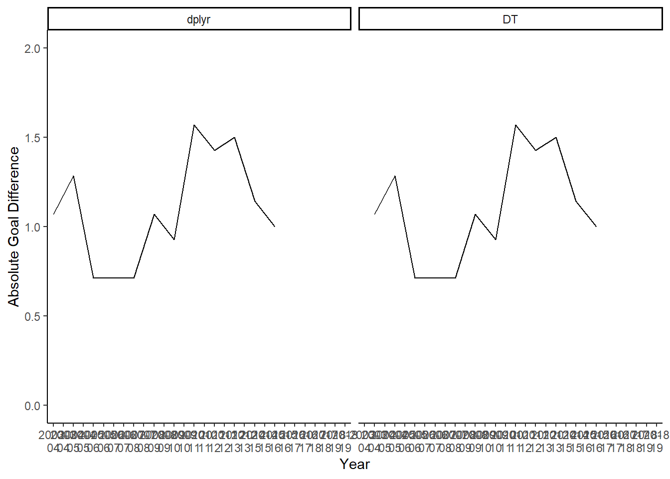
As we can see, the gap has been increasing, and is dramatically higher more recently. However, we do not know when the discrepancies are occurring. Are they occurring during the Round of 16, where there may be great discrepancies between the teams.
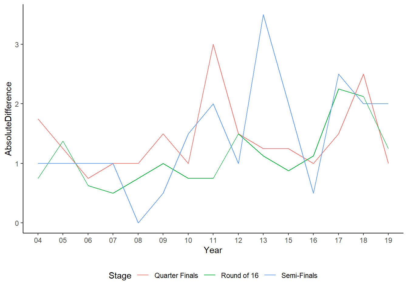
The gaps for all rounds increases overtime. There is a considerable amount of variation, but Round 16 is pretty consistent, although the gap is growing.