Using Python and Reticulate:
Reticulate is a R package that allows us to implement python within an R markdown file. This post shows how to do some basic predictive analysis using the same NBA dataset we used in prior posts.
We first need to read in the data. Below is some basic code to bring in a csv file.
import pandas as pd
import numpy as np

AnalyticalDS = pd.read_csv('NBAData/AnalysisDS.csv')
The plot below shows the distribution of minutes played for all players who were active. The code below is R. It shows the distribution of the minutes played variable mp. We use minutes played instead of seasons because it is a better representation of longevity than seasons.
However, the R plot shows both:
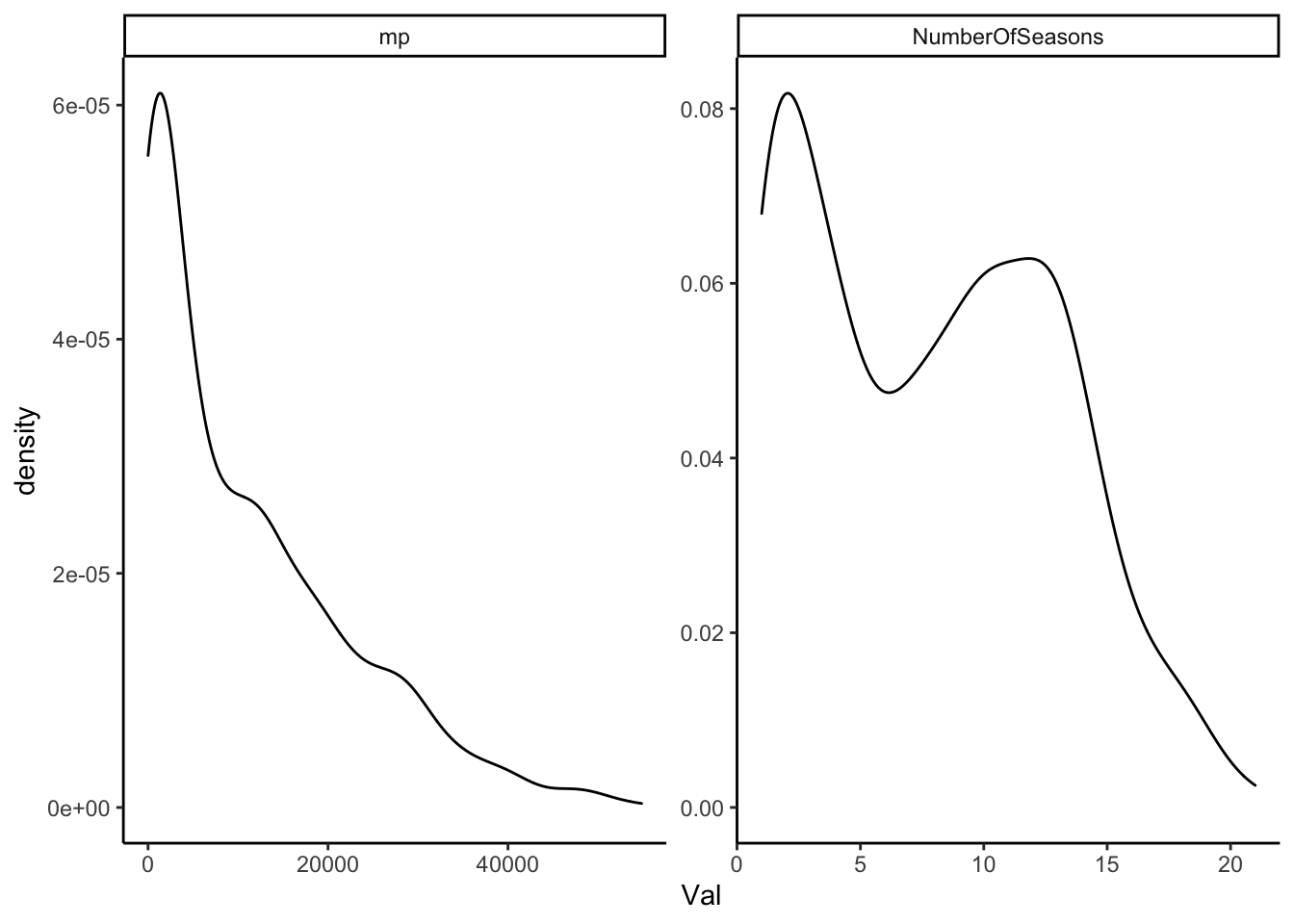
The next section code shows the same two plots but in python. As far as I can tell, there is not a perfect substitution for facet_wrap with scale = 'free'. You can import a python module ggplot, but that seems to defeat the purpose. The major advantage of scales = 'free' is that you show the distrbution for two very different variables.
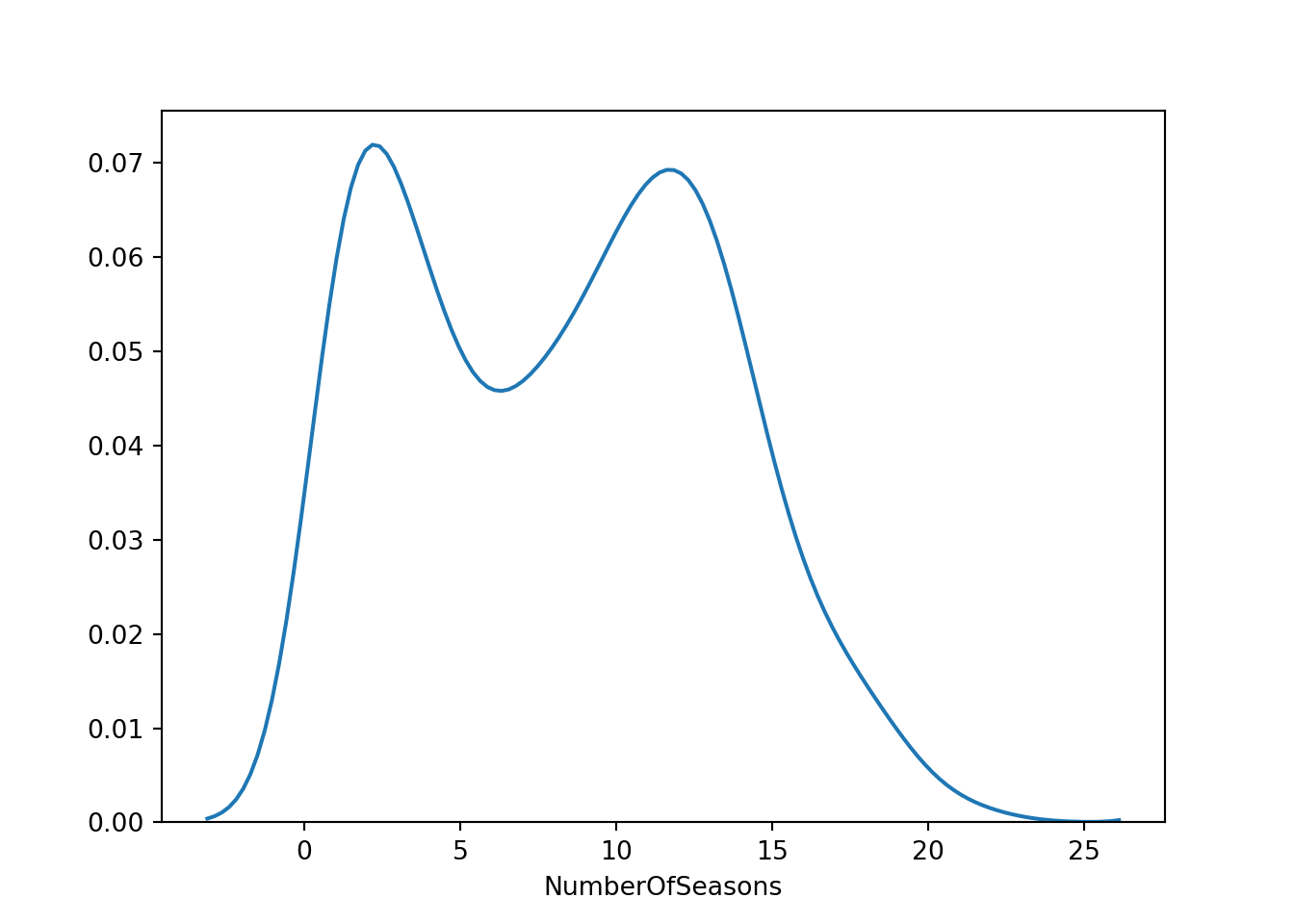
Instead, we use the seaborn module to show the same plots:
The first plot shows the distplot function for minutes played. The second plot is the same, but for NumberOfSeasons.
import seaborn as sns

sns.distplot(AnalyticalDS['mp'], hist = False)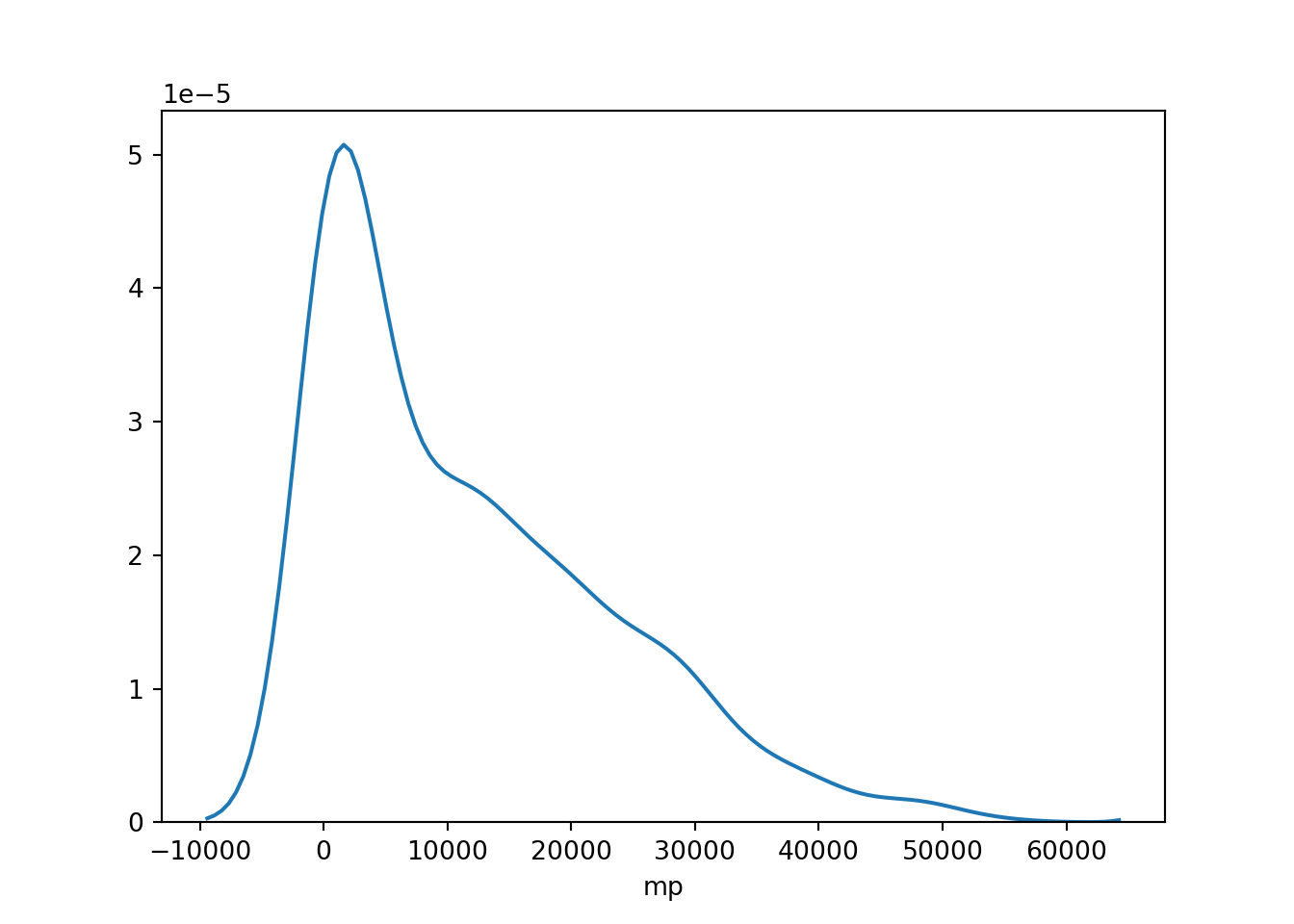
The next step is to finalize the dataset, the training dataset, and then the testing dataset. We first need to select the variables of interest, and then divide the data up. The below code removes any active players and players who had zero minutes. It also selects the variables we will need for our analysis.
AboveMP_zero = AnalyticalDS['mp'] > 0
NotCurrent = AnalyticalDS['LastSeason'] != "2019-20"
AnalyticalDS_2 = AnalyticalDS[AboveMP_zero]
AnalyticalDS_2_a = AnalyticalDS_2[NotCurrent]
## /Users/rebeccashapiro/Library/r-miniconda/envs/r-reticulate/bin/python:1: UserWarning: Boolean Series key will be reindexed to match DataFrame index.AnalyticDS_3 = AnalyticalDS_2_a[['link' ,'mp', 'age', 'FirstSeasonMP', 'fg', 'fga', 'ftpercent', 'FirstSeasonMP', 'PickNumber', 'fga', 'x3p', 'x3pa', 'x3ppercent', 'x2p' ,
'x2pa', 'x2ppercent', 'fgpercent', 'ft', 'fta', 'efgpercent', 'orb', 'drb', 'trb', 'ast', 'stl', 'blk', 'tov', 'pts','wprev', 'w_lpercentprev', 'wcur', 'w_lpercentcur']]This next section make the float variable PickNumber a categorical variable, and then a dummy variable with pandas module, using the function get_dummies. We then scale our continuous variables with a mean of zero, and a standard deviation of one.
Finally, we divide our data into a training and test datasets.
## /Users/rebeccashapiro/Library/r-miniconda/envs/r-reticulate/bin/python:1: SettingWithCopyWarning:
## A value is trying to be set on a copy of a slice from a DataFrame.
## Try using .loc[row_indexer,col_indexer] = value instead
##
## See the caveats in the documentation: https://pandas.pydata.org/pandas-docs/stable/user_guide/indexing.html#returning-a-view-versus-a-copy
The first algorithm we use is a ramdom forest. There is a very good description of how the algorithm actually works is here. There are many ways to evaluate a random forest algorithm; however, we will not do that here. It is possible to visualize a tree, and look at the Variable Importance. For an extensive discussion, see here.
The basic idea of a random forest is that it aggregates decision trees. Bagging uses a decision tree on a different dataset with sample with replacement technique.
Lasso
The next technique uses a lasso regression. Lasso regressions are unstable, which means that they do not consistently select the same features. Random forests are far more stable, which is a big advantage. To get out around the unstable nature of Lasso, we first try to bootstrap the lasso regression. We simply use 100 bootstraps for this example. Lasso is a simple linear regression, but with an extra parameter for shrinkage. Shrinkage attempts to minimize the parameters towards zero.
The final comparison is uses a simple grouped mean. We take the mean by the category of draft pick. A high draft pick, medium draft pick, etc…
The goal is to at least outperform the basic grouped mean.
The final table shows that the bootstrapped lasso performs the best. The metric is simply the mean absolute error.
| Model Name | Mean Absolute Error |
|---|---|
| Random_Forest | 6953.654 |
| Bootstrapped_Lasso | 6805.126 |
| Lasso | 6817.436 |
| Baseline | 9742.516 |
Summary
The post is pretty simple in that it takes three methods, and attempts to use some basic supervised learning to best predict minutes played among a group of NBA players who are no longer active.
We use a random forest and a lasso regresion, and a third method that uses the lasso algorithm, but with a bootstrap. Overall, we find that the bootstrap lasso performs the best, as the above table can be seen above.