Analysis:
The purpose of this analysis is to evaluate the impact of our three weather metrics on new Covid-19 cases in California. The complete and large dataset can be found here.
The complete code for this post can be found here:.
The basic California model will hypothesize that the stages of each opening should increase new cases after a week. Similarly, weather should work in a similar pattern. Better weather should encourage more outdoor activity, and we should see a drop in cases up until a certain point. Temperature rises beyond a certain point will have a positive association with new cases as it encourages more indoor activity.
The first step is to determine the model. The main choices of the model are the lag number. Does the temperature three days prior have a greater influence on new Covid-19 cases than the temperature 13 days prior? Ideally, we would use a log likelihood model. However, the models are not nested, and thus we do not use a log likelihood test. A nested models contains the previous model within it.
As we can see, the model with a six day lag has the lowest AIC, and it will be the model we evaluate. The Mdl column just tells us whether it is an interaction model or not. The interaction model has an interaction between temperature and precipiation intensity.
| Lags | Mdl | Val |
|---|---|---|
| 06 | AICInt | 53957.28 |
| 09 | AICInt | 53960.57 |
| 05 | AICInt | 53961.45 |
| 11 | AICInt | 53964.61 |
| 10 | AICInt | 53965.55 |
| 04 | AICInt | 53966.48 |
After deciding on the number of lags, we try modeling an interaction between temperature and precipitation intensity. We also try a second order polynomial as previously described.
The best model is the model with an interaction, and the second order polynomial. We use a likelihood ratio test, as all three models are nested.
After deciding on the model, we use a Bayesian work flow. Unfortunately, there is not enough computing power to check all of the lags, which is why we previously used a Frequentist work flow.
The next step is model a prior. Ideally, one can use institutional knowledge to determine the prior. For this modeling exercise, we will use the function get_prior from the brms package to determine the prior. As a comparison, we also use a weak prior. All of the parameters have been transformed to have a mean of zero, and a standard deviation of one.
We use the brms function model_weights. The model_weights provides a weighting system which judges the predictive accuracy of the posterior distribution. For a more extensive discussion, see here.
The model weights are based on the Widely Applicable Information Criterion (WAIC). For a very good explanation and detailed breakdown, see: here.
The below table shows the results.
| Model Evaluation | |||
|---|---|---|---|
| Models | elpd_diff | se_diff | ModelWeights |
| CovidBayesianStdCensus | 0.000 | 0.000 | 0.814 |
| CovidBayesian10Census | -1.704 | 0.944 | 0.148 |
| CovidBayesian10 | -3.621 | 5.020 | 0.022 |
| CovidBayesianStd | -3.939 | 4.951 | 0.016 |
As we can see there is not a considerable difference between the models. The elpd difference is smaller, or a similar size to the standard error. The model weights show that the CovidBayesianStdCensus model is the best model, but there is not a considerable difference between any of the four models. There is little difference between a weak, normally distributed prior, and Student’s T prior. There is also little difference between the addition of the census variables, and the model that does not have the census variables.
Checking the models:
Before looking at the credible intervals, and the mean estimate from the posterior distribution of our two temperature variables, we need to check the chains.
The chains for all of the models can be found here. There are four trace plots.
As we can see the chains follow the caterpillar like shapes. To do these plots, we follow the great Soloman Kurtz book, which is a tidyverse version of Statistical Rethinking by Richard McElreath.
library(bayesplot)


  TraceOut = mcmc_trace(dget("WeatherData/PosteriorDistr") %>%
                          filter(Model == "CovidBayesianStdCensus") %>% select(-Model) ,
             facet_args = list(ncol = 3),
             size = .15) +
    labs(title = paste0("Trace Plots for Model: CovidBayesianStdCensus" )) +
    theme_classic() +
    theme(legend.position = c(.95, .2))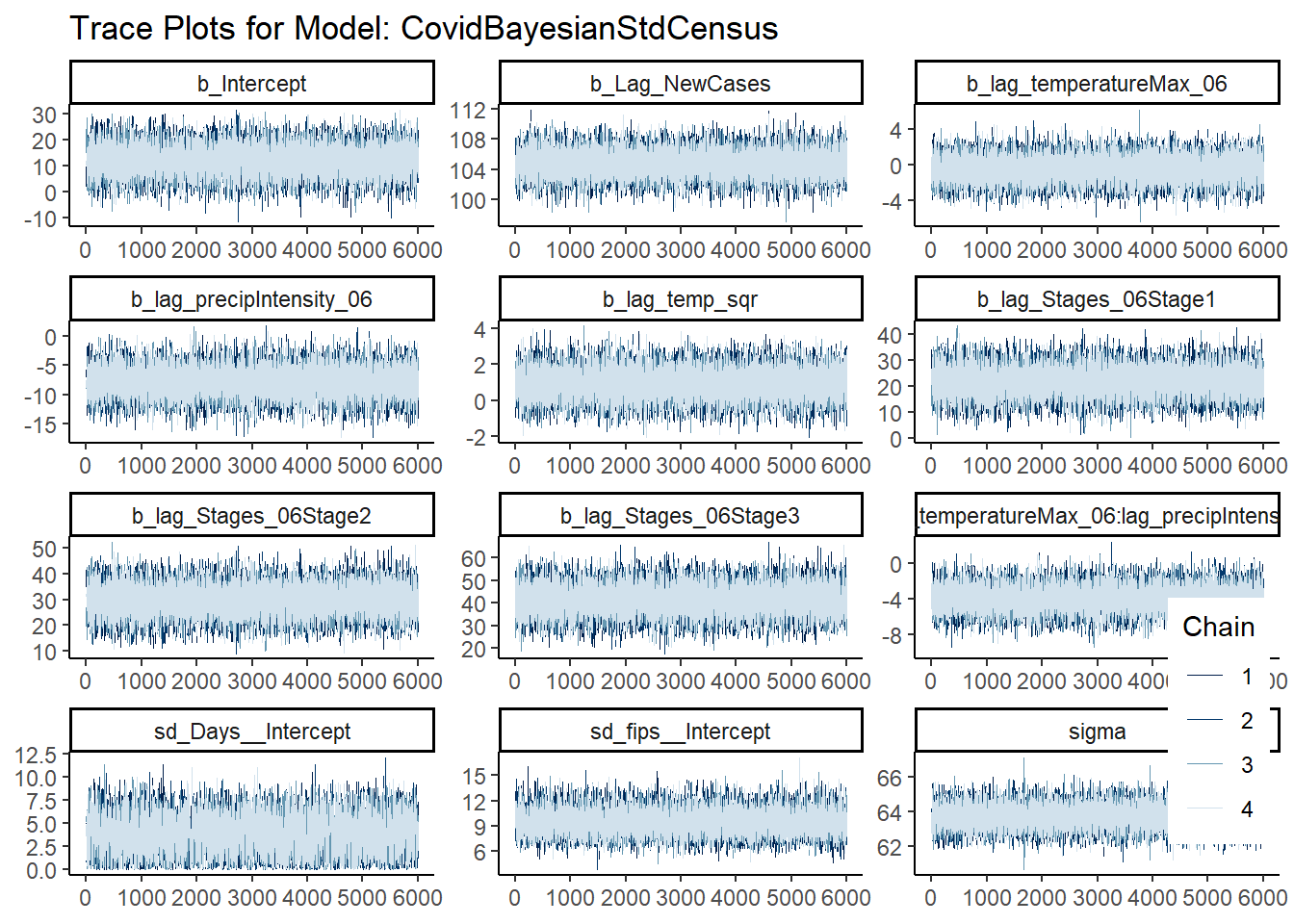
Analysis:
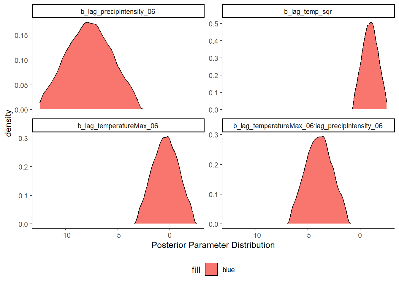
Next, we look at the posterior distribution of our parameters of interest, the weather variables. When we look at the posterior distribution for the weather variables, we see that the 95% credible intervals include zero for lag_temperatureMax_06 and lag_temp_sqr. The other two weather variables are the interaction between temperature and precipitation intensity, and the lag of precipitation intensitylag_precipIntensity_06. The credible intervals for both of these variables exclude zero.
All of the models can be found here.
The best model combination was the interaction model, where we modeled an interaction between the max temperature on a given day, and the precipitation intensity. In Statistical Rethinking, Richard McElreath notes that plotting interactions is a much more intuitive method to understand the effect.
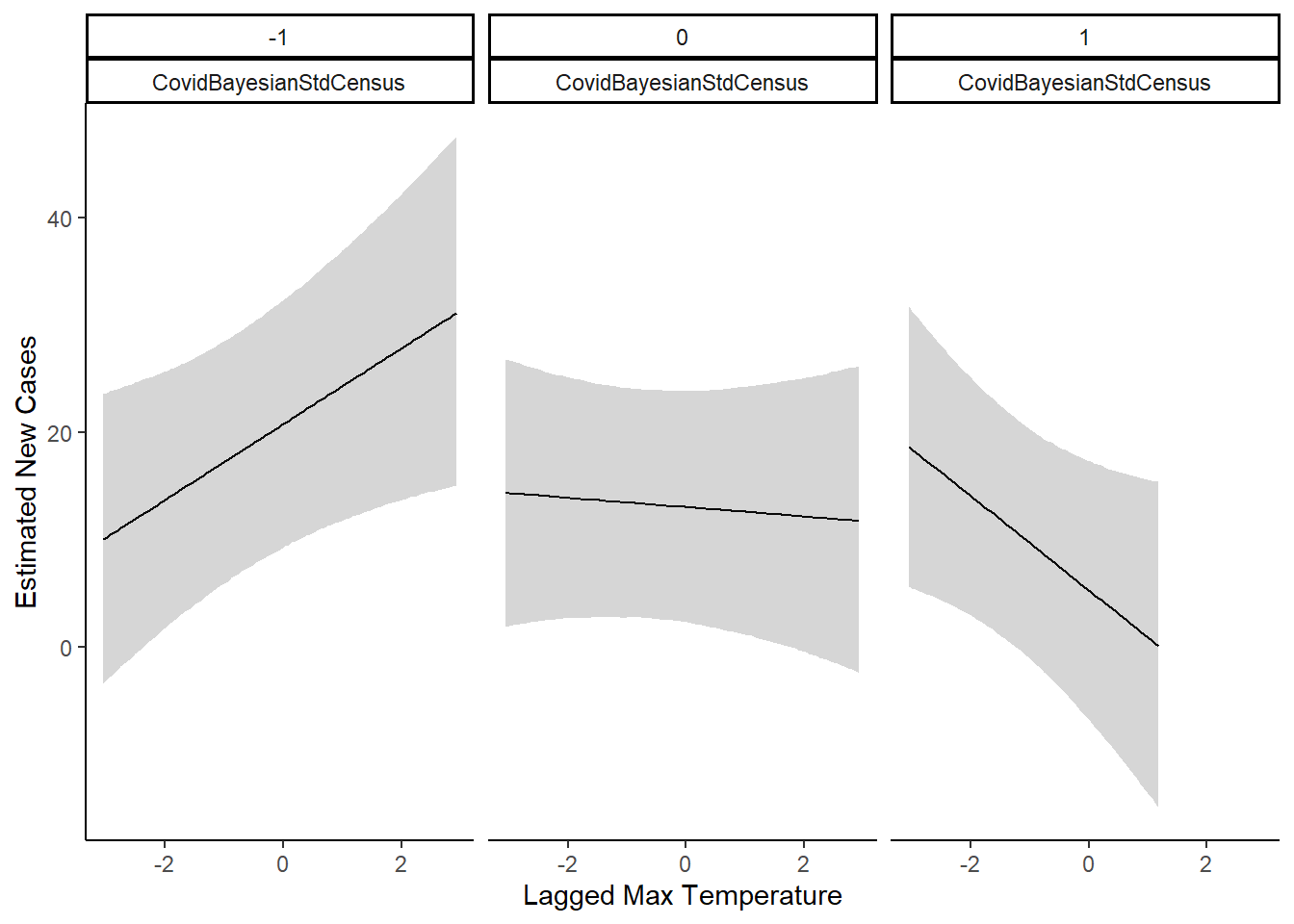
The plot above shows the interaction effect. When precipitation intensity is one standard deviation below mean, we see that as temperature increases, the estimated new cases rises. However, when precipitation intensity is one standard deviation above the mean, we see opposite. As temperature rises, estimated new cases decline. When precipitation intensity is at the mean, then temperature has little effect on estimated new cases.
Limitations and Conclusions
Overall, there is an effect of weather on the new cases in California. To summarize the interaction effect, good weather is associated with an increase in new cases.
However, there are major limitations. The dataset does not have testing numbers per day. Better weather may be correlated with an increase in testing, which in turn, would lead to more new cases discovered. Testing data would significantly improve this analysis.