The two previous posts have described the data available. This post will look to survival analysis to assess time until the end of a NBA career.
The code can be found here.
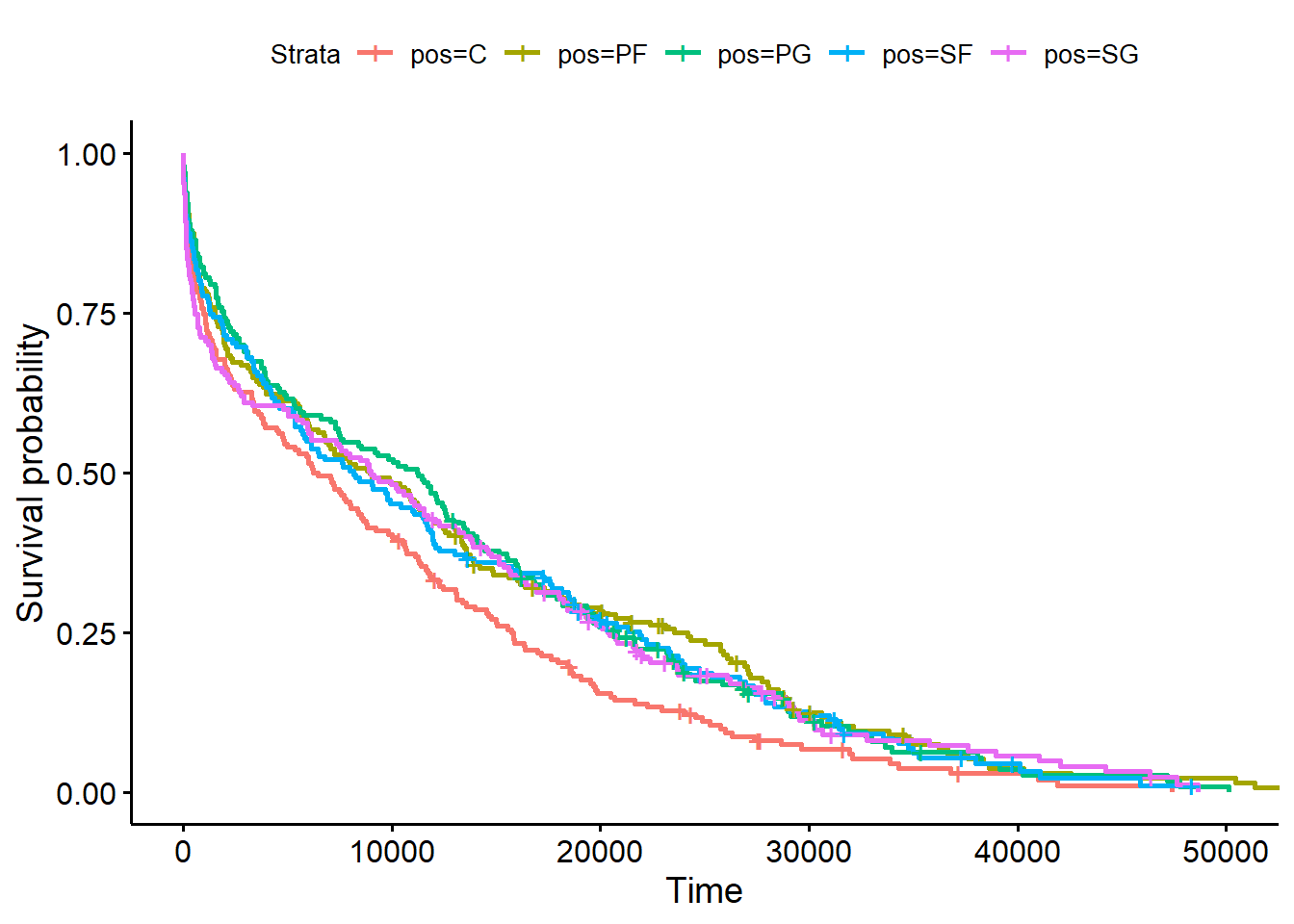
The first plot looks at the Kaplan Meier curves for both minutes played and seasons played by position.
As we can see, there is not a considerable difference between positions for the minutes played Kaplan-Meier curve.
Next, we look at the seasons played:
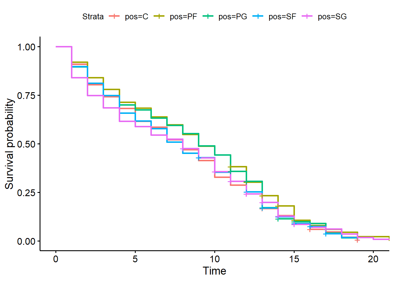
The green and blue curves are higher than the other three curves. This suggests that players classified as small forward, and point guard have longer careers.
While both metrics are interesting, minutes played better describes a players career arc. The following analysis will look at minutes played.
Cox Proportional Hazard:
The next step is to develop a regression model. We model hazard ratios.
With Basketball-Reference, there are basically infinite combinations of models we could consider. One method to develop this model could be to put all the possible factors that influence time until retirement, and use a lasso regression to determine which variables are best. However, there are problems with consistency with lasso regressions, see here:
Finally, we could use institutional knowledge. Institutional knowledge of how the Data Generated Process works allows us to use knowledge in an area to model a process. In this case, we understand that players who are better, get longer contracts, and can usually play longer as their skills atrophy.
Data
To model minutes, we will do so based on the players first season. We are not interested in how a given player performs in their fifth year, but rather, based on the first season in the NBA, what is the players expected career length as defined by minutes played. Minutes played is a good benchmark for both contracts, but also accounts for skill atrophy within a contract.
The variables of interest will be player statistics after their first year. We will consider both traditional statistics like points, assists, and rebounds, and more modern statistics like expected field goal percentage. A previous post showed how to pull draft position. We will also use draft position. Finally, we will test whether the first team a player plays on influences the length of their career.
After pulling each of the players season, we standardize all numeric variables. Andrew Gelman has a post about this here. In short, when comparing predictors within models, it is very useful to standardize the predictor variables as it allows us to look to see which predictors are the most predictive. To standardize variables in R, we use the function scale.
Lasso method:
To run the glmnet function, we need to create a matrix. We need the categorical variables to be dummies.
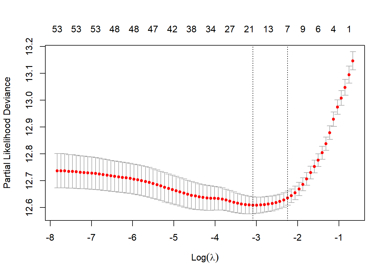
The plot below shows the lambda on the x-axis, and the partial likelihood deviance on the y axis. The goal is to minimize the partial likelihood deviance.
As an exercise, the below code shows how to reproduce the above plot with ggplot.
tibble(Likelihood = LassoReg$cvup,
       Lambda= LassoReg$lambda ) %>%
  mutate(LogLambda = round( log(Lambda) , digits = 0)) %>%
  ggplot(., aes(x = LogLambda, y = Likelihood)) +
  geom_smooth() +
  theme_classic() +
  geom_vline(xintercept =  log(LassoReg$lambda.min)) +
  labs(x = expression("Log"~(lambda)) ,
y = "Partial Likelihood Deviance") 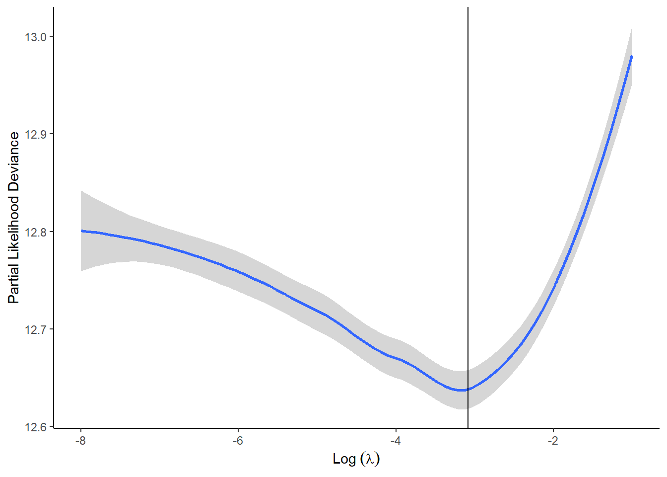
The minimum value of lambda is 0.0457228.
Using Institutional Knowledge
Institutional knowledge models use expertise and literature to develop a model. In this case, we will use expertise from NBA experts to develop a model.
The model will use the following predictors:
- Age - the younger a player, the longer they have to develop, and the longer their peak performance may be.
- Five year average of win-loss rate of first team. The theory is that better teams are more sound decision makers.
- Free throw percentages: a free throw percentage is a very good predictor for young players, as it shows their innate shooting skills.
- Free throw attempts: players who are able to get free throws can generate efficient offense.
- Effective Field Goal Percent: This just shows how efficient a basketball player is.
- Draft position – the higher a draft position, the better a given player is perceived to be by experts.
- Blocks and steals are very crude metric of defensive ability. f
- Points - simply because players with more points may be able to play longer because of reputation.
The team was excluded from this analysis. Team management changes over time, and the 5-year moving average of their win percentage is a better reflection of the organization of the team, then just the dummy variable of team.
Proportional Hazard Assumption
A key assumption in a Cox Proportional Hazard model is that that the proportional. This assumption simply states that the ratio of hazards must be constant over time. To check whether this assumption holds, we do two things:
- Check whether the interaction between time (minutes in our case) and the predictors are statistically significant.
For the Lasso model, there are two predictors which do not meet the proportional hazard assumption:
For the institutional model, there are three predictors which do not meet the proportional hazard assumptions.
| Proportional Hazard Table | ||
|---|---|---|
| term | Model | |
| Institutional | Lasso | |
| mp:blk | -1e-05 (0.01808871) | - |
| mp:FirstSeasonMP | - | 2e-05 (0.00011898) |
| mp:ft | -3e-05 (< 2.22e-16) | - |
| mp:fta | 3e-05 (< 2.22e-16) | 1e-05 (0.03879601) |
| mp:trb | - | -2e-05 (4.7254e-05) |
- Show the model’s Schoenfeld residuals plotted against time, or in this case, minutes played.
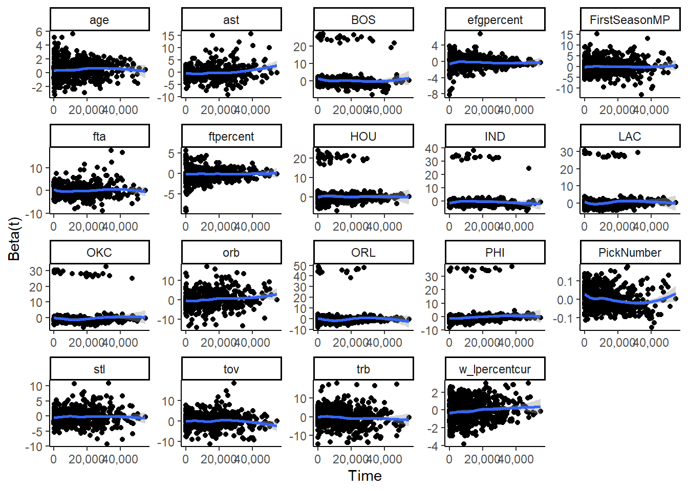
The above plot shows the Schoenfeld residuals against time for the Lasso model, and below is the plot shows the Schoenfeld residuals against time for the Institutional model.
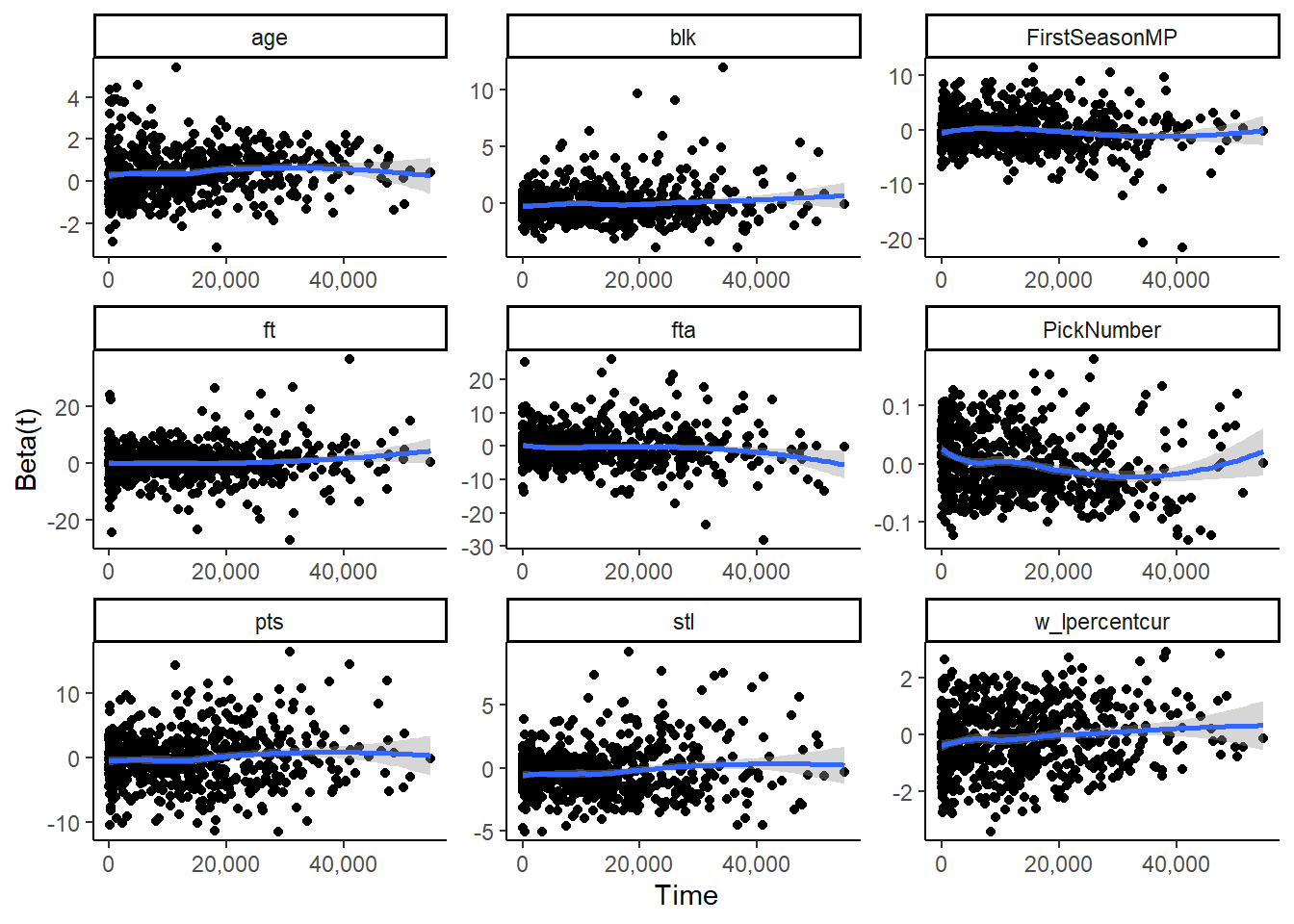
To resolve the violation of proportional hazards, we include an interaction between the variable which violates the proportional hazard assumption and the time variable, mp in our models.
Picking a model:
Survival models do not have provide a prediction the same way a logistic model. Comparing models based on prediction accuracy is not as viable.
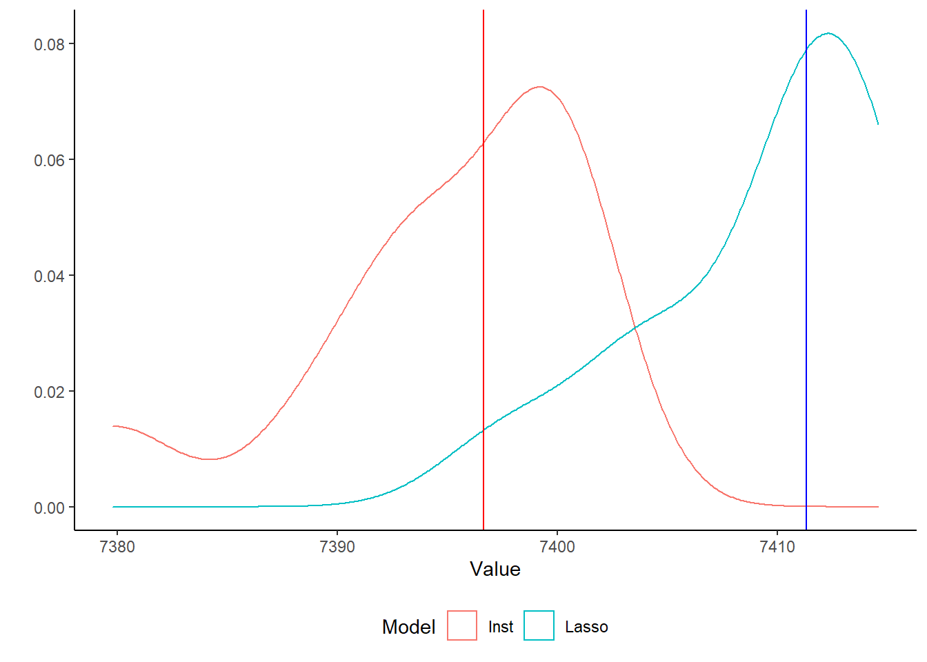
There is no perfect model to evaluate survival models. To evaluate the two models, we will follow this post. We will take 100 bootstraps, and calculate the AIC for each of the models. We then compare the median AIC for both models based on the 100 bootstraps.
Below is the plot of the 100 bootstraps. As we can see, the institutional model has a lower mean AIC value. Based on this limited exercise, this shows the value even limited knowledge of a field can have in model selection.
Final Model
The hazard ratios, and their confidence intervals an be found below:
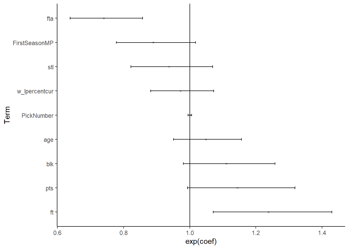
There are only two terms where the 95% confidence intervals do not include one.
First, an increase of one standard deviations of free throws is associated with a 24% increase in minutes played after adjusting for the other predictors.
Second, an increase of on standard deviations of free throw attempts is associated with a 26% decrease in minutes played after adjusting for other predictors.
Limitations:
This is obviously a short blog post on this topic. There is no information on contracts, player earnings, injuries, all of which are much clearer determinants of minutes played in a career than any of the predictors used.
Furthermore, this is not a predictive model. This model is a descriptive model which attempts to understand what factors best explain why players who played during the era of 2003 to 2010 played as many minutes as they did over the course of their career.
Summary
This post attempts to understand NBA player longevity through Cox models, and comparing two methods of model selection. The first model selection method uses Lasso regression, a form of supervised learning, to find the best model. The second model uses institutional knowledge to select the model.