Getting draft data
An interesting aspect of evaluating average player length is looking at their original draft position. The below code uses Basketball Reference and rvest to pull the drafts from 1985 to 2010.
This post uses the two packages rvest and the tidyverse package.
The code below looks through the NBA draft pages on Basketball Reference. It pulls the html tag table.
When the code reads in the data, the first few variables do not have assigned variable names. To quickly fix this, we use the janitor package, and the function clean_names. This gives each variable a name, and allows us to manipulate the dataset.
DraftDataReadIn = tibble(DraftYear = seq(1984, 2010, 1)) %>%
  mutate(URL = purrr::map(
    DraftYear, ~read_html(
      paste0("https://www.basketball-reference.com/draft/NBA_", .x, ".html")) %>%
      html_nodes("table") %>%
      html_table() %>%
      .[[1]]) )

DraftData = DraftDataReadIn %>%
  mutate(DraftData = purrr::map(URL, ~.x %>%
                                  janitor::clean_names() %>%
                                  select(2:5) %>%
           purrr::set_names(c("PickNumber", "Team", "PlayerName", "College")) %>%
             filter(row_number() > 1))) %>%
  select(-URL) %>%
  tidyr::unnest(DraftData)
Below is a table of how the data looks after the pull from Basketball Reference with a few data steps. The table shows the top five picks from the famous 1984 NBA draft.
| Top ten 1984 draft picks | ||||
|---|---|---|---|---|
| DraftYear | PickNumber | Team | PlayerName | College |
| 1984 | 1 | HOU | Hakeem Olajuwon | Houston |
| 1984 | 2 | POR | Sam Bowie | Kentucky |
| 1984 | 3 | CHI | Michael Jordan | UNC |
| 1984 | 4 | DAL | Sam Perkins | UNC |
| 1984 | 5 | PHI | Charles Barkley | Auburn |
| 1984 | 6 | WSB | Melvin Turpin | Kentucky |
Working with the draft data
The podcast the NBA redraftables frequently mention the Win Shares per pick, or per draft. As an example, we can use the 26 drafts pulled from above to see the most valuable picks based on Basketball Reference’s Win Shares and Player Efficiency Rating (PER).
To get these data, we again have to use the rvest package. While the code is not significantly more verbose, it is a little more challenging. The html_nodes function pulls the div tag. The html_text function removes all of the html from the pull, leaving just the text. This allows us to find the Win Share and PER values from the Basketball Reference.
AllPlayers = dget("NBAData/CompleteDataSet")

AllDistinctPlayers = AllPlayers %>%
  distinct(link) %>%
  mutate(GetPERWS = purrr::map(link, ~read_html(
      paste0("https://www.basketball-reference.com" , .x))  %>%
      html_nodes("div div") %>%
  html_text() %>%
  as_tibble()  %>%
  filter(grepl("\nPER", value) == TRUE | grepl("\nWS", value) == TRUE) %>%
    mutate(VarNm = stringi::stri_replace_all_regex(value, "[^[A-Z]]", ""),
         Number = gsub("\n|PER|WS", "", value)) %>%
  filter(VarNm %in% c("PER", "WS")) %>%
  select(-value) %>%
  tidyr::spread(VarNm, Number))) %>%
  tidyr::unnest(GetPERWS)
The plot below shows the Win Shares by pick number. Unfortunately, as you get further down the draft, there are fewer players that even make the NBA. Pick number 57 is a perfect example. There are only five picks from 1984 to 2010 that made the NBA, and were still playing between 2003 and 2010. Manu Ginobli is an elite player picked number 57. The average is not actually reflective of the impact of the 57 pick.
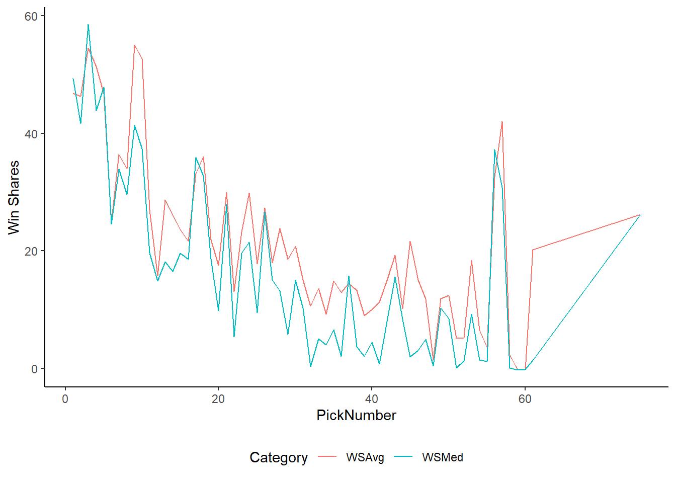
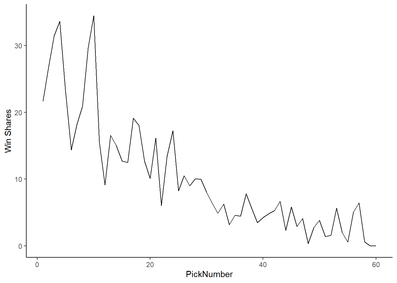
We can normalize this by just dividing the sum of Win Shares by the number of years of drafts. In this case, we looked at 26 drafts. We can divide the sum of win shares by pick number by 26. It is important to note that there is no pick number where there are 26 picks at the number are still in the league. For instance, there are 15 number one picks from 1984 to 2010 which played at least one season in the league between 2003 and 2010.
Finally, a violin plot shows the distribution of Win Shares by pick:
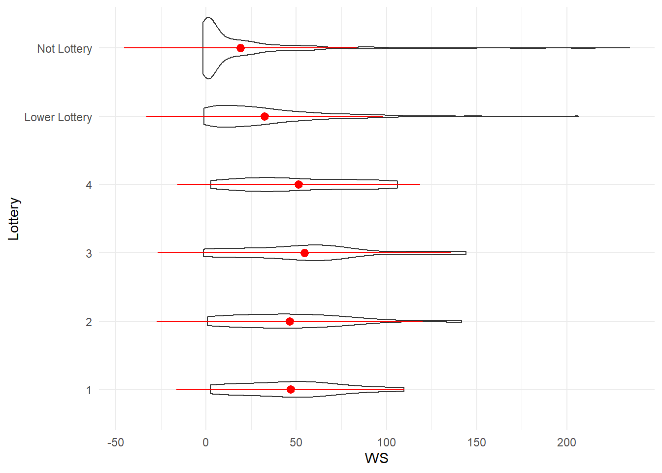
Overall, the top four picks have a similar mean. The third pick overall has the highest mean, but the fourth pick seems to have a greater share of its distribution further to the right of the Win Share axis. The lower lottery, and non-lottery picks have both lower means, and a greater share of their distribution near zero Win Shares.