The purpose of this post is to show how to use the ballr package to get historical NBA data, and after getting the data, find the best metric to use to determine longevity.
Ballr
The ballr package provides easy to use function to access the vast data resources on basketball-reference.com.
To get historical data for a defined group of players, we first pick a few given seasons. For our example, we pick the 2003 to the 2010 seasons.
The complete code to reproduce this post can be found here
Per36 = purrr::map( as.list(seq(2003, 2010, 1)) , ~ NBAPerGameStatisticsPer36Min(season = .x) ) %>%
  bind_rows(.)


PullLinksMissing = Per36 %>%
  select(player, link) %>%
  filter(is.na(link)) %>%
  distinct(player) %>%
  tidyr::separate(player, into = c("First", "Last"), remove = FALSE ,sep = "[ ]") %>%
  mutate_all(tolower) %>%
  mutate_at(vars(Last) , ~ stringi::stri_replace_all_regex(.x, "[^[:alpha:]]", "")) %>%
  mutate(newLink_a = paste0("players/" , stringi::stri_sub(Last, 1, 1) , "/",
                          stringi::stri_sub(Last,1,5),
                          stringi::stri_sub(First, 1, 2))  ,
         newLink = dplyr::case_when(First == "ray" & Last == "allen" ~ paste0(newLink_a, "02.html" ),
                             TRUE ~ paste0(newLink_a, "01.html")) ,
         FullURL = paste0("http://www.basketball-reference.com/", newLink))  %>%
  rowwise() %>%
  mutate(Exist = url.exists(FullURL)) %>%
  ungroup() %>%
  mutate(ShortenURL = stringi::stri_replace_all_fixed(FullURL,
                                                      "http://www.basketball-reference.com", "")) %>%
  mutate(PlayerInfo = purrr::map( ShortenURL,  NBAPlayerPerGameStats) ) %>%
  select(player,link=ShortenURL, PlayerInfo)

dput(PullLinksMissing,"MissingPlayers")

PullLinksCompl = Per36 %>%
  filter(!is.na(link)) %>%
  select(link, player) %>%
  distinct(link, .keep_all = TRUE) %>%
  mutate(PlayerInfo_a = purrr::map( link,  NBAPlayerPerGameStats) ,
         PlayerInfo = purrr::map(PlayerInfo_a , ~ .x %>% mutate_at(vars(-season, -tm, -lg, -pos), as.numeric)) )
The first step is to pull all player data for these years. We use the function NBAPerGameStatisticsPer36Min, and only keep the distinct player names and links. In the dataset, there is a variable called link, which provides the URL to that player on Basketball Reference.
Note, there are some players who do not have a link. After googling, and using some intuition, I realized the players were all hall of famers. The asterisks in the underlying data break the link function from the ballr package.
To fix this, we use the url.exists function from the RCurl package to recreate the URL. The link the function NBAPlayerPerGameStats is basically the following:
- players
- the lowercase first letter of the last name
- the first five letters of the last name
- the first two letters of the first name
- a digit which refers to whether a player who has the same name preceded that player. For instance, for Ray Allen, there was another Ray Allen. His digit is 02, while most other players have 01.
Finally, after getting our unique links for both players who have a links, and players who do not, we pull the full career statistics for all players from 2003 to 2010 using NBAPlayerPerGameStats.
There is one final data issue. The class of each of the columns NBAPlayerPerGameStats pulls in is not consistent. Across the eight datasets (2003 to 2010), the variable games or g, is classified as both character and numeric. To resolve this final issue, we simply define all variables as numeric with the exception of a few variables prior to using the command unnest.
CompleteDataSet = bind_rows( PullLinksCompl , PullLinksMissing ) %>%
  mutate(PlayerInfo2 = purrr::map(PlayerInfo , ~ .x %>%
                                    mutate_at(vars(-season, -tm, -lg, -pos), as.numeric))) %>%
  select(-PlayerInfo) %>%
  tidyr::unnest(PlayerInfo2)

dput(CompleteDataSet , "CompleteDataSet")
Take a look at the data:
Now that we have the data, we can look at the average length of a career, average minutes, among other variables that represent basketball playing career.
There are 949 unique players in the dataset.
There are four variables that we could use to define length of career:
- Starting age to ending age.
- Number of games
- Number of minutes
- Number of seasons
We’ll show the distribution for each of these below:
Starting Age:
The starting age to ending age shows the journey. A player like PJ Tucker may have entered the league at age 21, but then did not play again until the age of 27. He is now thriving at age 35. The duration of his career includes seasons played in Europe. Basketball Reference data does not capture that.
The first plot looks at the distribution of the three age metrics. The dashed-red vertical line is the median value of each of the three metrics. This plot includes active players, or more specifically, players who have an entry for the 2019-2020 season.
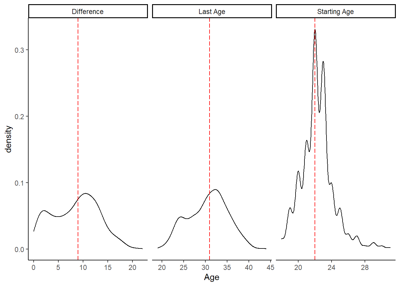
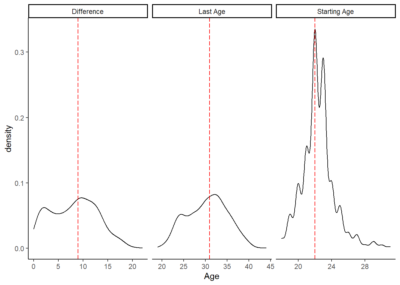
The second plot is the same, however, we remove active players.
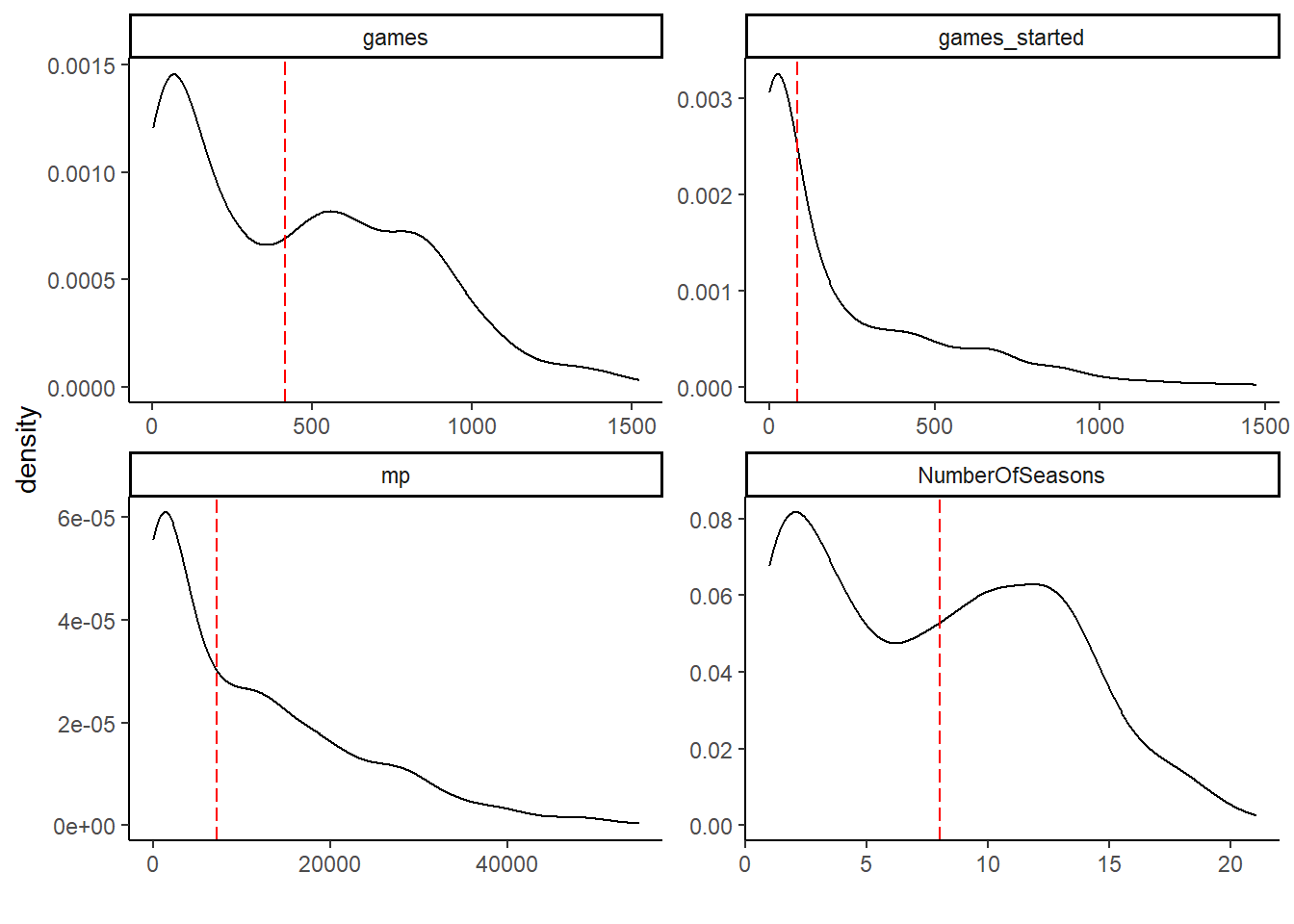
Number of Minutes and Games Played
The number of games played is conceptually simple idea. However, it is hard to differentiate between a player who had low minutes played because of injuries, and a player who had low minutes played because of poor performance.
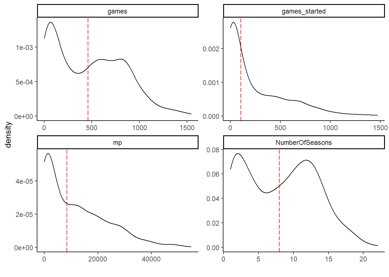
Including, or excluding current players does not change the distribution in particular.
Summary
Overall, the ballr package is intuitive to use, and using a couple of functions together can provide a powerful mechanism to pull lots of career data from Basketball-Reference. This post looked at different longevity metrics for player careers. Overall, minutes played, or mp is probably the best metric as it provides information on length of career and quality of career.